The Excel XLOOKUP function is a modern and flexible replacement for older functions like VLOOKUP, HLOOKUP, and LOOKUP. XLOOKUP supports approximate and exact matching, wildcards (* ?) for partial matches, and lookups in vertical or horizontal ranges.
- lookup – The lookup value.
- lookup_array – The array or range to search.
- return_array – The array or range to return.
- not_found – [optional] Value to return if no match found.
- match_mode – [optional] 0 = exact match (default), -1 = exact match or next smallest, 1 = exact match or next larger, 2 = wildcard match.
- search_mode – [optional] 1 = search from first (default), -1 = search from last, 2 = binary search ascending, -2 = binary search descending.
XLOOKUP is a modern replacement for the VLOOKUP function. It is a flexible and versatile function that can be used in a wide variety of situations.
XLOOKUP can find values in vertical or horizontal ranges, can perform approximate and exact matches, and supports wildcards (* ?) for partial matches. In addition, XLOOKUP can search data starting from the first value or the last value (see match type and search mode details below). Compared to older functions like VLOOKUP, HLOOKUP, and LOOKUP, XLOOKUP offers several key advantages.
Not found message
When XLOOKUP can’t find a match, it returns the #N/A error, like other match functions in Excel. Unlike the other match functions, XLOOKUP supports an optional argument called not_found that can be used to overide the #N/A error when it would otherwise appear. Typical values for not_found might be “Not found”, “No match”, “No result”, etc. When providing a value for not_found, enclose the text in double quotes (“”).
Note: Be careful if you supply an empty string (“”) for not_found. If no match is found, XLOOKUP will display nothing instead of #N/A. If you want to see the #N/A error when a match isn’t found, omit the argument entirely.
Match type
By default, XLOOKUP will perform an exact match. Match behavior is controlled by an optional argument called match_type, which has the following options:
| Match type | Behavior |
|---|---|
| 0 (default) | Exact match. Will return #N/A if no match. |
| -1 | Exact match or next smaller item. |
| 1 | Exact match or next larger item. |
| 2 | Wildcard match (*, ?, ~) |
Search mode
By default, XLOOKUP will start matching from the first data value. Search behavior is controlled by an optional argument called search_mode, which provides the following options:
| Search mode | Behavior |
|---|---|
| 1 (default) | Search from first value |
| -1 | Search from last value (reverse) |
| 2 | Binary search values sorted in ascending order |
| -2 | Binary search values sorted in descending order |
Binary searches are very fast, but data must be sorted as required. If data is not sorted properly, a binary search can return invalid results that look perfectly normal.
Example #1 – basic exact match
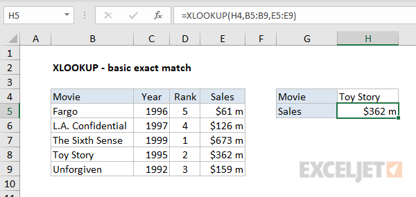
By default, XLOOKUP will perform an exact match. In the example below, XLOOKUP is used to retrieve Sales based on an exact match on Movie. The formula in H5 is:
=XLOOKUP(H4,B5:B9,E5:E9)

More detailed explanation here.
Example #2 – basic approximate match
To enable an approximate match, provide a value for the “match_mode” argument. In the example below, XLOOKUP is used to calculate a discount based on quantity, which requires an approximate match. The formula in F5 supplies -1 for match_mode to enable approximate match with “exact match or next smallest” behavior:
=XLOOKUP(E5,B5:B9,C5:C9,,-1)

More detailed explanation here.
Example #3 – multiple values
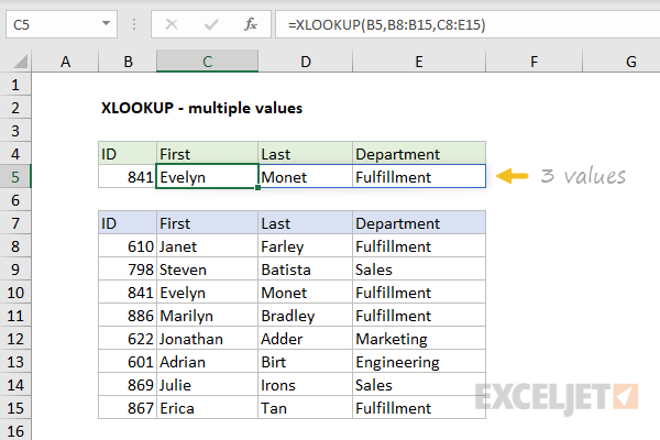
XLOOKUP can return more than one value at the same time for the same match. The example below shows how XLOOKUP can be configured to return three matchging values with a single formula. The formula in C5 is:
=XLOOKUP(B5,B8:B15,C8:E15)

Notice the return array (C8:E15) includes 3 columns: First, Last, Department. All three values are returned and spill into the range C5:E5.
Example #4 – two-way lookup
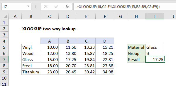
XLOOKUP can be used to perform a two-way lookup, by nesting one XLOOKUP inside another. In the example below, the “inner” XLOOKUP retrieves an entire row (all values for Glass), which is handed off to the “outer” XLOOKUP as the return array. The outer XLOOKUP finds the appropriate group (B) and returns the corresponding value (17.25) as the final result.

Example #5 – not found message
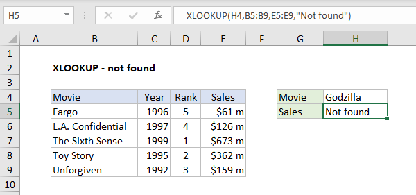
Like other lookup functions, if XLOOKUP does not find a value, it returns the #N/A error. To display a custom message instead of #N/A, provide a value for the optional “not found” argument, enclosed in double quotes (“”). For example, to display “Not found” when no matching movie is found, based on the worksheet below, use:
=XLOOKUP(H4,B5:B9,E5:E9,"Not found")

You can customize this message as you like: “No match”, “Movie not found”, etc.
Example #6 – complex criteria
With the ability to handle arrays natively, XLOOKUP can be used with complex criteria. In the example below, XLOOKUP is matching the first record where: account begins with “x” and region is “east” and month is not April:

